데이터 종류에 따른 추천시스템 모델 종류

1. User-Item Interaction → Collaborative Filtering Methods 사용

   ex) ratings or buying behavior

2. Attribute Information about the users and items → Content-based Methods 사용

   ex) textual profiles or relevant keywords, a single(not all) user’s rating

정의

Collaborative filtering models use the collaborative power of the ratings provided by multiple users to make recommendations

To address some of the limitations of content-based filtering, collaborative filtering uses similarities between users and items simultaneously to provide recommendations. This allows for serendipitous recommendations; that is, collaborative filtering models can recommend an item to user A based on the interests of a similar user B. Furthermore, the embeddings can be learned automatically, without relying on hand-engineering of features

Explicit, Implicit

Explicit

Users specify how much they liked a particular movie by providing a numerical rating

Implicit :

If a user watches(행동) a movie, the system infers that the user is interested

Customer preferences are derived from their activities rather than their explicitly specified ratings

When a customer buys(행동) an item, it can be viewed as a preference for the item. However, the act of not buying an item from a large universe of possibilities does not always indicate a dislike

단점

1. The underlying ratings(or feedback) matrices are sparse

   In the movie cases, most users would have viewed only a small fraction of the large universe of available movies

   → 해결책:

   • CSR Matrix
   • Linked List Matrix(LIL)
2. Cannot handle fresh items
3. Hard to include side features for query/item

Collaborative Filtering의 두 가지 방식

Memory-based Collaborative Filtering

※ Nearest neighborhood-based(최근접이웃기반) Collaborative Filtering이라고도 함

These algorithms are based on the fact that similar users display similar patterns of rating behavior and similar items receive similar ratings

→ Target User가 아직 평가하지 않은 아이템을 Target User와 유사한 User집단들의 평가의 기반으로 예측하는 것이 목표!

Methods

1. User-based collaborative filtering 방법

   한 아이템에 대한 추천 정도를 측정하려면 해당 아이템에 대해 평점을 내렸던 유저들 전체 중에서 나와 유사도가 높은 유저들만 추려 해당 아이템을 어떻게 평가하고 있는지 확인하는 방법

   The ratings provided by like-minded users of a target user A are used in order to make the recommendations for user A

   Similarity functions are computed between the rows of the ratings matrix to discover similar users

   	ItemA	ItemB	ItemC	ItemD	ItemE
   User1	3	4	4		1
   User2	4	4	4	3
   User3	1	1	2	5

   ※ 주황색 : 유사도가 높음

   ※ 테이블 해석 : User1과 User2는 ItemA, B, C까지 평점 유사도가 높다

2. Item-based collaborative filtering 방법

   In order to make recommendations for target item A, the first step is to determine a set S of items, which are most similar to item A. Then, in order to predict the rating of any particular user4 for item A, the ratings in set S, which are specified by user4, are determined. The weighted average of these ratings is used to compute the predicted rating of user A for item B

   Similarity functions are computed between the columns of the ratings matrix to discover similar items

   When such methods are applied to the transpose of the ratings matrix, they are referred to as item-based neighborhood models

   	User1	User2	User3	User4	User5
   ItemA	5	4	4		5
   ItemB	4	4	4	5
   ItemC	1	1	2	3

   ※ 주황색 : 유사도가 높음

Distinction Between User-based and Item-based

The ratings in user-based CF are predicted using the ratings of neighboring users, whereas the ratings in item-based CF are predicted using the user’s own ratings on neighboring (i.e., closely related) items.

In the user-based CF case, neighborhoods are defined by similarities among users (rows of ratings matrix), whereas in the item-based C case, neighborhoods are defined by similarities among items (columns of ratings matrix)

Strengths and Weaknesses of Neighborhood-Based Methods

1. Advantages

   • Simplicity and intuitive approach.

     It is often easy to justify why a specific item is recommended, and the interpretability of item-based methods is particularly notable

   • Relatively stable with the addition of new items and users

2. Disadvantage
   • Least O(m2) time and space.

   • Limited coverage because of sparsity

     For example, if none of John’s nearest neighbors have rated Terminator, it is not possible to provide a rating prediction of Terminator for John. On the other hand, we care only about the top-k items of John in most recommendation settings. If none of John’s nearest neighbors have rated Terminator, then it might be evidence that this movie is not a good recommendation for John. Sparsity also creates challenges for robust similarity computation when the number of mutually rated items between two users is small.

Model-based Collaborative Filtering

In model-based methods, machine learning and data mining methods are used in the context of predictive models. In cases where the model is parameterized, the parameters of this model are learned within the context of an optimization framework. Some examples of such model-based methods include decision trees, rule-based models, Bayesian methods and latent factor models. Many of these methods, such as latent factor models, have a high level of coverage even for sparse ratings matrices

Data Matrix

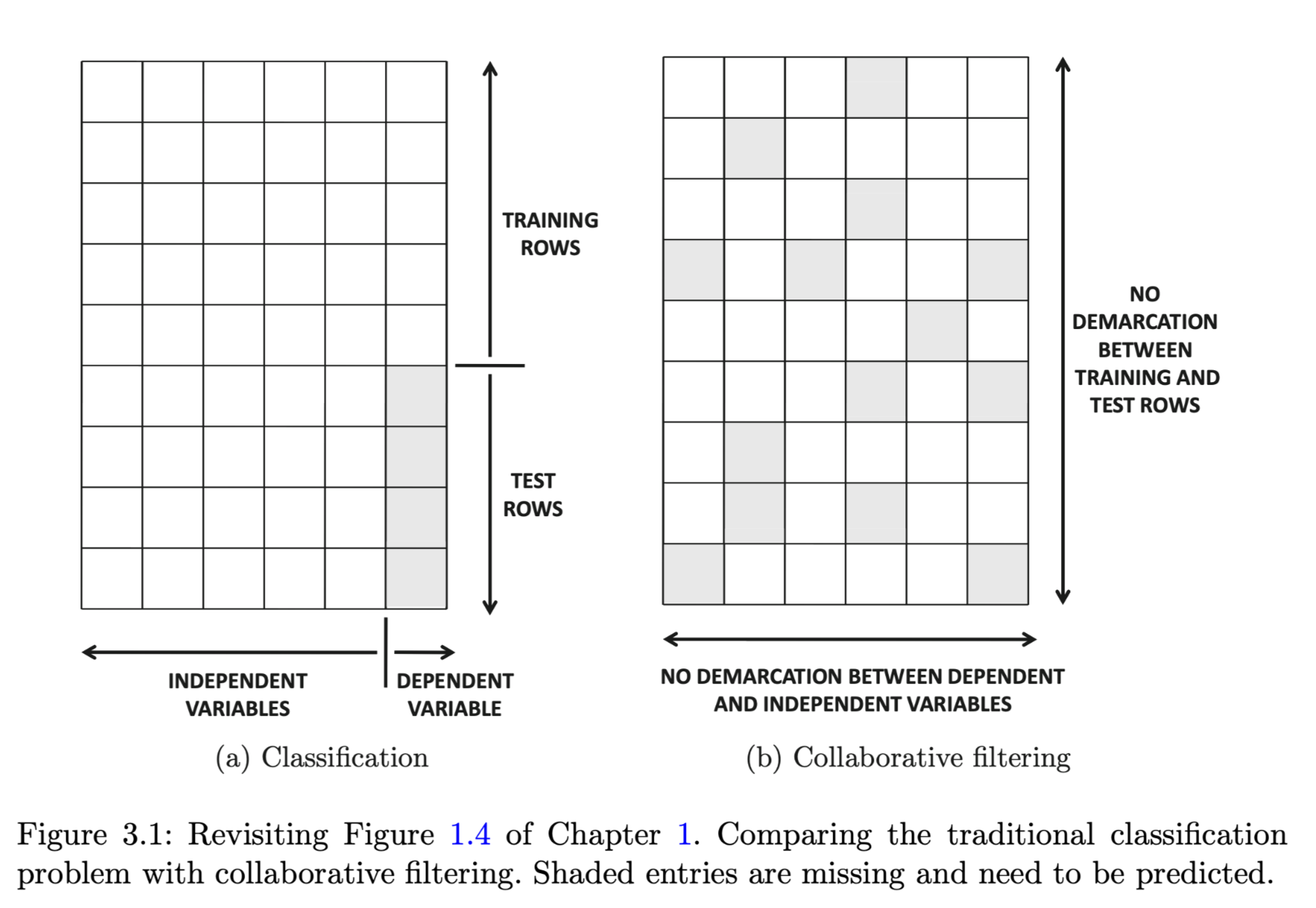
1. Data Classification problem

   we have an m × n matrix, in which the first (n − 1) columns are feature variables (or independent variables), and the last (i.e., nth) column is the class variable (or dependent variable). All entries in the first (n − 1) columns are fully specified, whereas only a subset of the entries in the nth column is specified. Therefore, a subset of the rows in the matrix is fully specified, and these rows are referred to as the training data. The remaining rows are referred to as the test data. The values of the missing entries need to be learned for the test data. This scenario is illustrated in Figure 3.1(a), where the shaded values represent missing entries in the matrix.

   Columns represent features, and rows represent data instances

2. Collaborative Filtering Problem

   Any entry in the ratings matrix may be missing, as illustrated by the shaded entries in Figure 3.1(b). Thus, it can be clearly seen that the matrix completion problem is a generalization of the classification (or regression modeling) problem

   The specified (observed) entries to be the training data, and the unspecified (missing) entries to be the test data.

Advantages

1. Space-efficiency:

   Typically, the size of the learned model is much smaller than the original ratings matrix. Thus, the space requirements are often quite low. On the other hand, a user-based neighborhood method might have O(m2) space complexity, where m is the number of users. An item-based method will have O(n2) space complexity.

2. Training speed and prediction speed:

   One problem with neighborhood-based methods is that the pre-processing stage is quadratic in either the number of users or the number of items. Model-based systems are usually much faster in the preprocessing phase of constructing the trained model. In most cases, the compact and summarized model can be used to make predictions efficiently.

3. Avoiding overfitting:

   Overfitting is a serious problem in many machine learning algorithms, in which the prediction is overly influenced by random artifacts in the data. This problem is also encountered in classification and regression models. The summarization approach of model-based methods can often help in avoiding overfitting. Furthermore, regularization methods can be used to make these models robust.

Types for Model-based CF

• Decision and Regression Tree to Collaborative Filtering
• Rule-based Collaborative Filtering
• …
• Latent Factor Models
• …

→ 다음은 Model-based CF 중 Latent Factor Models에 대해 설명함

Latent Factor Models

The goal is to use dimensionality reduction methods to directly estimate the data matrix in one shot

Dimensionality Reduction

These models leverage well-known dimensionality reduction methods to fill in the missing entries. Dimensionality reduction methods are used commonly in other areas of data analytics to represent the underlying data in a small number of dimensions. The key idea in dimensionality reduction methods is that the reduced, rotated, and completely specified representation can be robustly estimated from an incomplete data matrix. Once the completely specified representation has been obtained, one can rotate it back to the original axis system in order to obtain the fully specified representation. Under the covers, dimensionality reduction methods leverage the row and column correlations to create the fully specified and reduced representation. For example, user-based neighborhood methods leverage user-wise correlations, whereas item-based neighborhood methods leverage item-wise correlations

Intuition for understanding Latent Factor Model

(1) Geometric Intuition

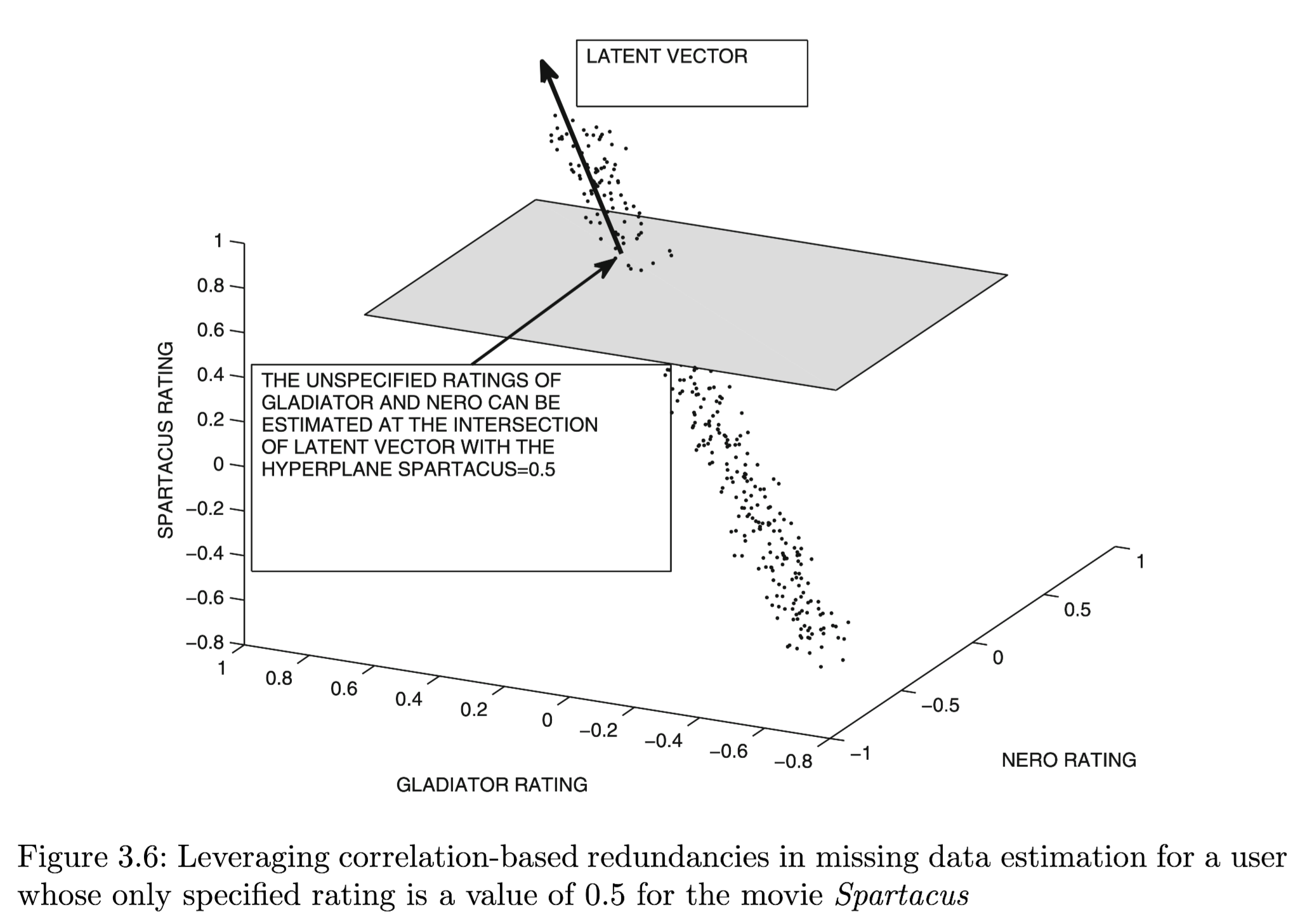
→ 이후 설명은 이해할 수 없었음. 다음에 다시 확인해봐야겠다

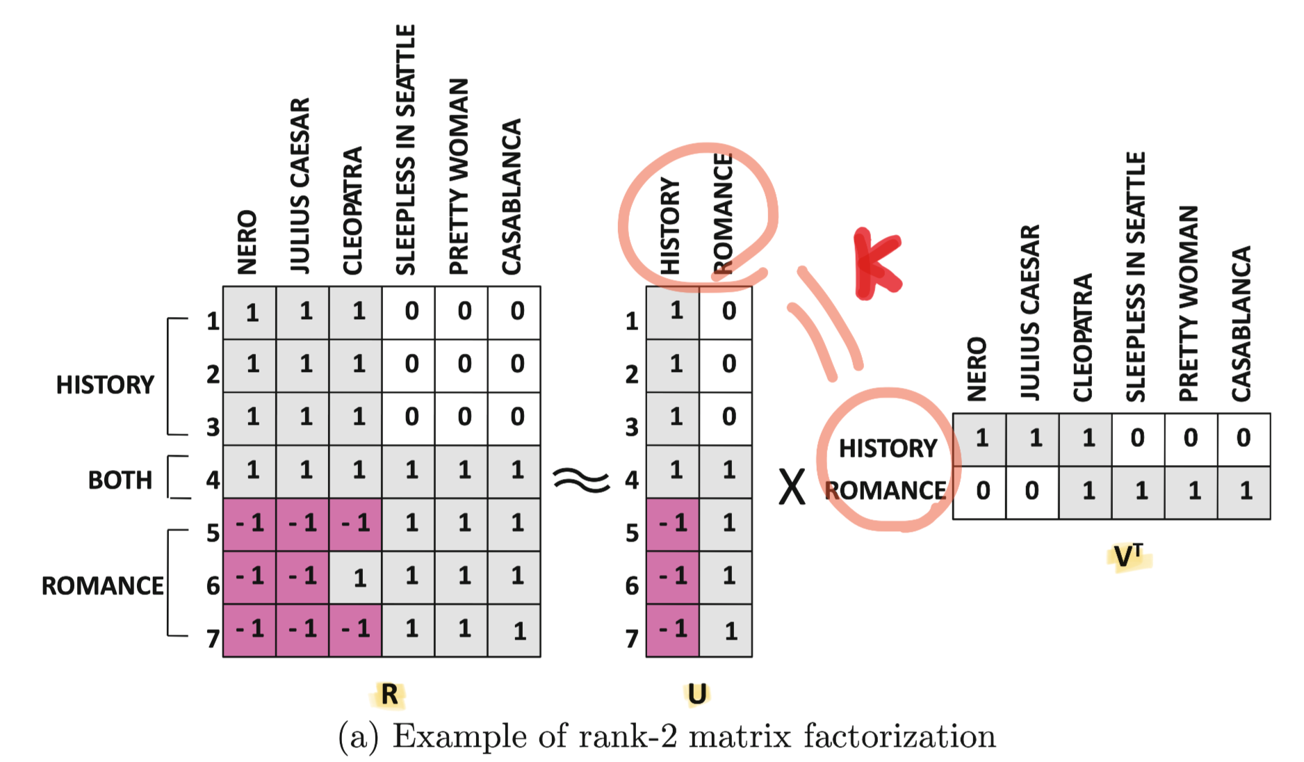
(2)Low-Rank Intuition

\[R = UV^T\]

• $U=m \times k$
• $V = n \times k$
• The rank of both row space and the column space of $R$ is $k$

→ 이후 설명은 이해할 수 없었음. 다음에 다시 확인해봐야겠다

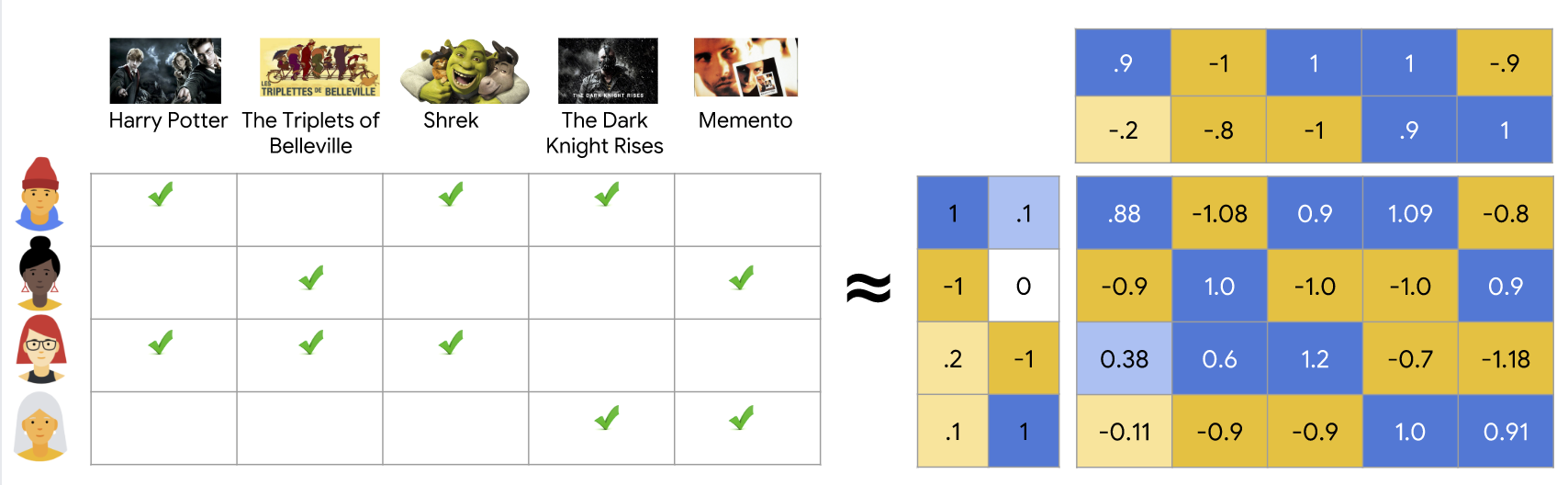
Matrix Factorization(MF)

Matrix factorization methods provide a neat way to leverage all row and column correlations in one shot to estimate the entire data matrix

Most dimensionality reduction methods can also be expressed as matrix factorizations

The goal of matrix factorization is to find the optimal feature vectors that minimize the difference between the estimated ratings and the actual ratings

Basic Principles of MF

1. Formula

$ R \approx UV^T $

• \[A \in R^{\ m \times n}\]

  , where $m$ is the number of users(or queries) and $n$ is the number of items

• Latent Vector/Component: Each column of $U$ (or $V$)

  A latent vector may often be an arbitrary vector of positive and negative values and it becomes difficult to give it a semantic interpretation. However, it does represent a dominant correlation pattern in the ratings matrix

• Latent Factor : Each row of $U$ (or $V$)

  • User Factor: Each row $\bar{u_i}$ of $U$

    It contains $k$ entries corresponding to the affinity of user $i$ towards the $k$ concepts in the ratings matrix

  • Item Factor : Each row $\bar{v_i}$ of $V$

    It represents the affinity of the $i$th item towards these $k$ concepts

    

1. Each Rating Value($r_{ij}$)

\[r_{ij} \approx \bar{u_i} \ \cdot \ \bar{v_i}\]

• $\bar{u_i}= (u_{i1}\dots u_{ik})$
• $\bar{v_j}= (v_{j1} \dots v_{jk})$

\[r_{ij} \approx \Sum^k_{s=1}u_{is} \ \cdot \ v_{js}\] \[= \Sum^k_{s=1}(\text{Affinity of user i to concept s}) \ \times (\text{Affinity of item j to concept s})\]

Complexity

Matrix factorization typically gives a more compact representation than learning the full matrix. The full matrix has $O(nm)$entries, while the embedding matrices $U, V$ have $O((n+m)d)$ entries, where the embedding dimension $d$ is typically much smaller than $m$ and $n$

As a result, matrix factorization finds latent structure in the data, assuming that observations lie close to a low-dimensional subspace. In the preceding example, the values of n, m, and d are so low that the advantage is negligible. In real-world recommendation systems, however, matrix factorization can be significantly more compact than learning the full matrix.

Advantage and Disadvantage of MF

Advantage

• Handle sparse and incomplete data

  MF can fill in the missing values and predict ratings for unseen items or users

• Reduce the dimensionality and complexity of the data

  MF can compress a large matrix into smaller matrices that capture the essential information and reduce the noise

• Discover latent features and patterns that are not obvious or explicit in the data

  MF can reveal hidden similarities and preferences among users and items, which can enhance the quality and diversity of the recommendations

Disadvantage

• Overfitting and underfitting

  To avoid these problems, matrix factorization needs to balance the trade-off between fitting the data and regularizing the feature vectors

• Sensitive to the choice of parameters

• Limited by the linearity and independence assumptions

  Matrix factorization assumes that the rating is a linear combination of the features, and that the features are independent of each other. However, in some cases, the rating may depend on nonlinear or interactive features, or on external factors such as context, time, or social influence. To address these limitations, matrix factorization may need to incorporate additional information or techniques, such as nonlinear functions, feature engineering, or hybrid models

Reference

• Recommender Systems(Charu C. Aggarwal)
• Collaborative Filtering - Google
• Matrix Factorization - Google
• MF Pros and Cons - Linkedin
• Matrix Factorization Techniques for Recommender Systems - Papers